
In his wildly popular 2015 Bloomberg article about
programming,
Paul Ford included a short section about what happens inside your computer
between pressing the “a”
key
and getting an a printed to the screen. His point was that even the most
straightfoward human instructions can become surprisingly delicate and complex
when filtered through wire and silicon, and that programmers are basically just
humans with the right constitution to brook the journey.
Coders are people who are willing to work backward to that key press.
— Paul Ford, “What is Code?”
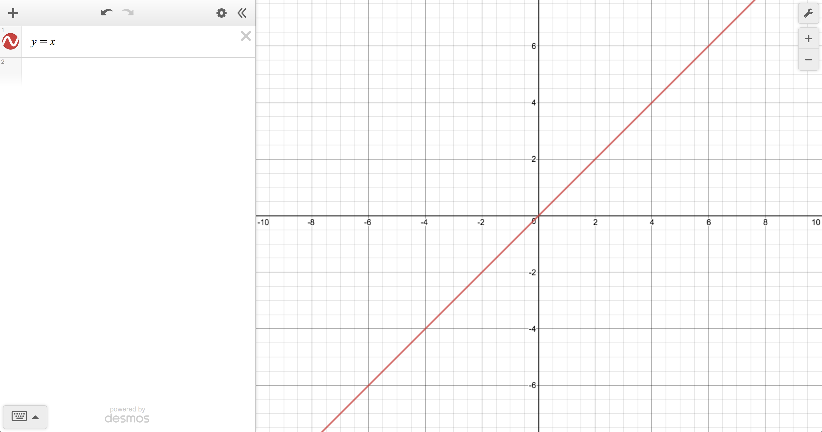
Today, I’d like to work forward from a key press inside the Desmos graphing calculator, following it through the cascade of changes it produces in order try to translate your mathematical instructions into pixels painted by a browser. In other words, what has to happen so that, when you press “x” inside of an expression, you eventually see this:
Housekeeping
Before we do anything mathematically interesting with your key press, we have to do a bit of housekeeping to determine whether or not it should even be mathematically interesting. The outcome of a key stroke in the calculator depends on its current context, so the first thing we do is make sure that its handling is delegated to the right part of the system. A top-level event listener checks against a list of keyboard shortcuts to see whether we should trigger some kind of special action, like undo/redo, opening the image upload dialog, or…displaying the list of keyboard shortcuts. We also have to deal with keyboard navigation so that, in particular, people who are using screen readers have a good experience.
Assuming your key press should result in a bit of new text, we immediately start the process of rendering it.
Rendering typeset math
I say “process” because most mathematical strings in the calculator are represented in LaTeX—so that we always have enough information to display them nicely—but requiring users to enter raw LaTeX is considered, outside of certain academic circles, an act of hostility. So this is where we temporarily hand over control to MathQuill, our awesome, open-source typesetting library.
One way MathQuill improves the situation is by transforming a sane sequence of
keystrokes into a bit of well formed LaTeX before doing anything else. For
example, pressing the / key will generate the string '\\frac{}{}' and not
'/'. MathQuill also does some helpful normalizations, such as automatically
matching grouping symbols, inserting \left and \right before delimiters so
they can be properly sized, and converting configurable text shortcuts into
valid LaTeX commands or operators. That’s how, in the graphing calculator,
'pi' becomes '\\pi' and 'sum' becomes '\\sum' so they can be rendered
as π and ∑, respectively.
MathQuill comes with its own LaTeX parser that returns a tree of what is
essentially the virtual DOM necessary for producing a visually correct layout.
After normalization and parsing, MathQuill goes about building the corresponding
actual DOM, takes a bunch of measurements so that all the relative sizing
works out, and adds the new nodes to the page. The net result is an element that
feels mostly like a native input (complete with a “cursor” that’s really just a
tiny blinking <span>) but contains beautifully typeset math instead of vanilla text.

And at this point we’re hitting the first visible side effects. Your new character is officially on the screen.
Dispatches from the front end
Once MathQuill has finished rendering, the view has to tell the rest of the
world what just happened. It dispatches a
Flux action that includes the input’s
current latex value in the payload, along with an id so that we know which
model should receive the update. The action’s type is determined by which sort
of input just changed. You may, for instance, be trying to update the viewport
window, or a point label, or part of a parametric domain.
For the sake of our example let’s assume, going forward, that you’re doing the most fundamental of Desmos things: updating a basic expression. In that case, the dispatch from the view will end up looking something like this:
// ExpressionView
handleLatexChanged(latex: string) {
  this.controller.dispatch({
    type: 'set-item-latex',
    id: this.id,
    latex,
  });
}
Since the only information we have at this point is the new LaTeX associated with the expression, we just optimistically update the model. We have no idea whether what you typed makes any sense, mathematically, but that’s a problem for Future Desmos to deal with.
function setLatex(model: ExpressionModel, latex: string) {
  // Beautifully typeset possible gibberish
  model.latex = latex;
}
Off the beaten thread
Until now everything has been happening on the main thread, which is mostly okay. Because MathQuill might end up taking a lot of measurements and causing a lot of reflows in order to handle dynamic sizing, it’s possible to bog down the UI if your expression gets crazy, but that’s usually not a huge problem in practice. Reasonably complicated expressions (and, actually, many unreasonably complicated ones) take tolerably long to render, and if you really want to DOS yourself with a mile-long continued fraction, we won’t get in your way. We’ll do our best to handle what you throw at us without imposing arbitrary limits (caveat emptor).
But after typesetting we’re headed into the teeth of the calculator’s business logic, where many computations can take long enough that, if we performed them on the main thread, we might have a hard time responding to further user actions, causing the UI to become laggy. To keep things feeling snappy, the next few steps of the process get passed off to web workers.
Parse, parse, lower
A change in an expression model’s latex triggers a request to the parser so
that we can turn a user-entered string into a parse tree that captures all of
the information needed by the math and plotting engines. Calling it “the parser”
is a little misleading, since it actually comprises three distinct passes wired
in series. The whole process warrants its own post, but here’s the basic outline:
- Convert the raw LaTeX into a display tree. The first pass captures the
notion of a visual “group” (for example, the numerator of a fraction or the
contents of a superscript or radical) and is essentially mathematically
ignorant. Different LaTeX strings that produce identical layouts should have
identical semantics (e.g.,
1+2*3and{1+2}*3). - Transform the display tree into an expression tree. The second pass transforms visual groups into a tree that captures arithmetic precedence in the form of “surface” nodes, which roughly means that they ignore how deep in the parse tree they are.
- “Lower” the expression tree. Finally, we transform the expression tree into one that contains more specific expression nodes based on their context and location within the parse tree. (For instance, this is where we determine whether two comma-separated values represent a list or an ordered pair.)
In code, the skeleton looks like this:
function parseLatex(input: string): DisplayTree;
function parseExpression(dTree: DisplayTree): ExpressionTree;
function lower(eTree: ExpressionTree, ctx: LowerCtx): ParseResult;

interface LowerCtx { /* some extra context about legal nodes */ }

function parse(input: string): ParseResult {
  const ctx: LowerCtx = { /* ... */ };
  const group: DisplayTree = parseLatex(input);
  const tree: ExpressionTree = parseExpression(group);

  return lower(tree, ctx);
}

// Example
parse('y=\\frac{1}{3}x+\\left[2,4,6\\right]');

/*
 * =>
 * Assignment(
 *   Identifier('y'),
 *   Add([
 *    Multiply([
 *      Divide([
 *        Constant(1),
 *        Constant(3)
 *      ]),
 *      Identifier('x')
 *     ]),
 *    List([
 *      Constant(2),
 *      Constant(4),
 *      Constant(6)
 *    ])
 * ]))
 */
Even though parsing could all technically be done in a single pass, separating
concerns like this makes the whole thing simpler to reason about and maintain.
Splitting (1) and (2) helps mitigate the fact that LaTeX precedence isn’t the
same as arithmetic precedence, and defining them separately reduces the
likelihood that those conflicts lead to actual problems. Splitting (2) and (3)
helps limit the amount of context the parser “core” needs to hold onto, which
means we can reuse it across several tools (or configurations) by writing
different lower implementations rather than writing different parsers.
Hello, calculator
If all this talk about parsing reminds you of programming languages, that’s good. An expression is really a tiny piece of program that we’ve just converted into a parse tree, and next we have to “compile” it into something that’s executable. Each parse node knows how to return a JavaScript function representation of itself, and that’s the function we call internally in order to produce an evaluated result or, in the case of plotting, many evaluated results.
Getting concrete
After parsing and compilation, we’re left with a tree of parse nodes, but it’s still abstract. For instance, nodes that were parsed as identifiers might actually be assigned concrete values in some other expression in the list, and we’ll need to know that in short order. So the next step is to generate a concrete tree by substituting concrete values from the “frame”—basically, a dictionary of all the exported definitions in the expressions list—for each abstract node. This is also the stage where we do constant collapsing where possible.
/*
 * Expressions:
 * a = 4
 * 2a + x
 */

// Abstract tree for '2a + x'
Add([
  Multiply([
    Constant(2),
    Identifier('a')
  ]),
  Identifier('x')
])

// Concrete tree after frame substitution
Add([
  Multiply([
    Constant(2),
    Constant(4)
  ]),
  FreeVariable('x')
])

// Concrete tree after constant collapsing
Add([
  Constant(8),
  FreeVariable('x')
])
Once we’ve turned your expression into a data structure that we can ask meaningful questions about—and which can even ask a few meaningful questions about itself—we have to figure out what we should do with it. There are a lot of possibilities, but the most salient decision is whether we should evaluate it, plot it, export a definition, or display an error (not all mutually exclusive).
Most of those cases are relatively straightfoward. The parser lets us know about errors early, and we propagate those back up the front end for display in the UI. (A pleasant side effect of the lowering phase is that we can generate extremely helpful error messages without having to cruft up the main parsing routine.)
Exporting a definition amounts to adding an entry to the frame, which is simple enough, but because the expressions list is basically a complete declarative program, there’s a chance that any frame update can cause changes in every expression. That means we have to restart the process of creating a concrete tree for each abstract tree, setting off a ripple of updates. We try to be clever about batching changesets.
If we determine that the expression should display an evaluation to the user, we call the top-level node’s compiled function and pass the result to the view. If that’s all that’s required (the analysis concludes that the expression shouldn’t produce any graphed output), the process ends here, with the calculator having calculated something and updated the view(s) in the expressions list.
The graphing part of the graphing calculator
If our analysis determines that your updated expression should draw something to
the graph paper, we have to decide among a couple of strategies for doing that,
based on some particulars of the expression’s form. We have roughly four
different plotting routines: one for functions of a single variable (like y =
x^2) and equations that are simple enough to solve for one variable or another
(like x + y - 1 = 0), one for implicit equations that are too complicated to
solve for either variable (like x cos(y) = y cos(x)), one for parametric
functions (like (cos(t), sin(t))), and one for polar equations (like r = θ).
At the most basic level, they each function roughly the same way: the compiled function is sampled at a discrete set of inputs, and the resulting points are used to form line segments that hopefully represent the behavior of the underlying continuous function with an acceptable level of accuracy. Where they differ is in how they choose and update those inputs. This is another topic that deserves its own post, but I’ll lay out some of the main ideas.
For the “simple” cases, we start with a bunch of evenly spaced on-screen values along one axis and evaluate the compiled function at each of those values, in order, to generate a point. Sequences of points that are nearly co-linear are collapsed to single straight segments to simplify plotting. If neighboring points suggest that there is a zero crossing, a local extremum, or a jump, we use bisection to try to find the location where one of these occurs as precisely as possible.

The polar and parametric plotters use the same basic process, with a couple of twists. The parametric plotter still samples a one-dimensional domain, but it has to evaluate two compiled functions, one for each coordinate. The recursive subsampling routine for parametrics is also adaptive so that we can be more sensitive to curvature. In the polar case, we try to determine whether or not the compiled function is periodic, as a performance optimization, so that we can avoid sampling and plotting the same curve over and over again.
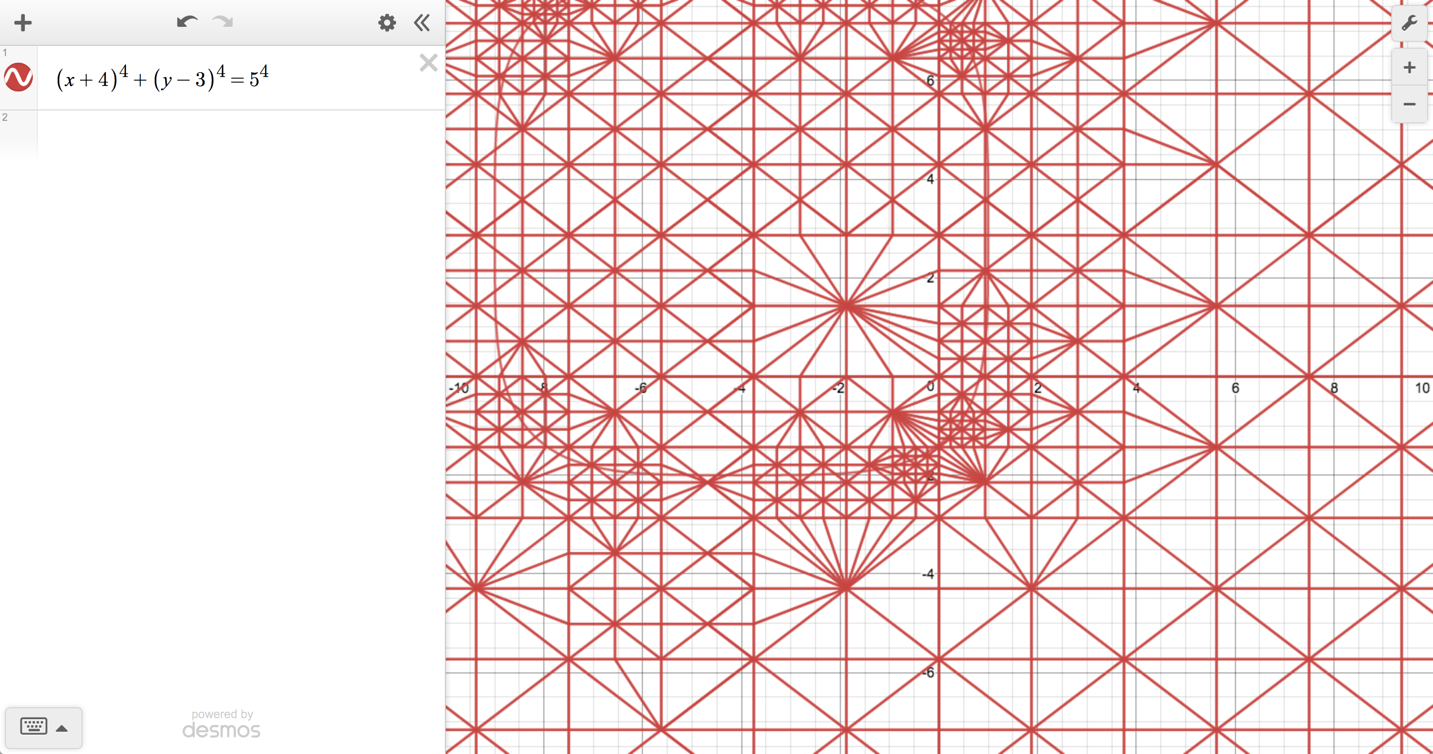
The implicit plotter is a different beast entirely because, instead of sampling from an interval, we have to sample from the entire plane. You can imagine normalizing an implicit equation by setting one side equal to 0, which leaves you with some expression in x and y on the other side. Substituting a point into that expression gives you a result that’s either 0 (a solution), positive, or negative. Rather than trying to find all of the solutions directly, our goal is to approximate the boundary between regions of positive and negative value, because the exact boundary is the solution set.
To do this, we initially choose points from the vertices of a quadtree, which can be subdivided to different depths for different regions, depending on where things get interesting. We then tile the quadtree with triangles such that their edges separate positive and negative regions of the plane. And, finally, we build up a polygon out of those triangle edges to represent the boundary curve.
Each method has its advantages and disadvantages (everything about doing math on computers is a compromise). We could, for instance, produce more accurate plots by always using the implicit plotter, but it tends to be slow relative to the other options because of its more complicated sampling behavior. One of Desmos’s primary goals is to make math feel interactive and exploratory, so we’re constantly looking for ways to strike a satisfying balance between speed and visual fidelity.
Regardless of which plotter we use, the end result is an array of tiny line segments that get passed back to the main thread. When we hear back from the worker, we combine the segment information with the current user preferences about color, line style, etc., and draw them to the canvas, completing the final leg of our trip.
What now?
There’s certainly a lot of ground to cover between the keyboard and the screen, but it’s really only half the story. What goes on between the screen and your brain is far more interesting to us. Ultimately, we want the graphing calculator to be a tool that helps everyone have a better relationship with math. We’ll keep working on our part of the journey in the hope that we can make yours a little more enjoyable. So, here’s the real question: Which key do you want to press next?
We’ll be waiting.