
Over the past year, Desmos has made major improvements to the robustness of regressions (i.e., fitting models to data) in the graphing calculator, particularly for trigonometric, exponential, and logistic models. This post will outline some of the challenges of solving regression problems and some strategies we have used to overcome those challenges.
Before and After
Let’s begin with a couple examples of regressions that have improved over the last year.
.png)
.png)
In this trigonometric regression, there are many possible combinations of parameters that all fit the data exactly equally as well. Notice the $R^2$ statistic is identical for the high-frequency fit that the calculator found previously and the low-frequency fit that the calculator finds today. But our intuition rejects the high-frequency fit: all else equal, we should prefer a lower frequency fit when its errors are exactly as small as a higher frequency fit. The calculator is now aware of this special rule.
.png)
.png)
In this logistic regression, the calculator previously got stuck in a region where small adjustments to the parameters $b$ and $c$ didn’t make any perceptible difference to the errors—the calculator was left with no good clues about what to try next. Notice that the true best fit value of one of the parameters, $b = 3.2\cdot10^{23}$, is pretty extreme. It can be difficult for the calculator to find regression parameters that are either extremely large or extremely small, but the calculator is now able to handle logistic regressions like this one much more reliably.
Both of these cases were especially frustrating because our eye tells us it should obviously be possible to find a better fit than the calculator was finding. Why didn’t it know what we know?
Easy Regressions and Hard Regressions
Roughly speaking, linear regressions are easy, and nonlinear regressions are hard.
Linear Regression
A linear regression is a regression that depends linearly on its free parameters. For example,
y_1 \sim m x_1 + b
is a linear regression model ($x_1$ and $y_1$ represent lists of data, and $m$ and $b$ are free parameters). The model
y_1 \sim a x_1^2 + b x_1 + c
is also a linear regression because it depends linearly on the free parameters $a$, $b$, and $c$. For the definition of a linear regression, it doesn’t matter that this model depends nonlinearly on the data $x_1$.
Nonlinear Regression
A couple common examples of nonlinear regression problems are the exponential model
y_1 \sim ab^{x_1},
which depends nonlinearly on the parameter $b$, as well as the trigonometric model
y_1 \sim a \sin(b x_1 + c),
which depends nonlinearly on the parameters $b$ and $c$.
Method of Least Squares
The calculator determines the best fit values of free parameters in both linear and nonlinear regression problems using the method of least squares: parameters are chosen to minimize the sum of the squares of the differences of the sides of a regression problem.
For example, in the linear regression problem
y_1 \sim m x_1 + b,
the total squared error, considered as a function of the free parameters $m$ and $b$, is
E(m, b) = \sum_{n} \left(y_1[n] - \left(m x_1[n] + b\right)\right)^2,
where I’m using the calculator’s notation that $y_1[n]$ is the nth element of the list $y_1$. In all linear regression problems, including this one, the error is a quadratic function of the free parameters.
The minimum of this error function can be found using a little bit of calculus and a little bit of linear algebra: differentiate the error with respect to each of its parameters and set each of the resulting partial derivatives equal to zero. The derivatives are all linear functions of the parameters, so this produces a system of $n$ linear equations in $n$ unknowns that can be solved as a single linear algebra problem using matrix techniques.
Linearizing and Iterative Methods
In nonlinear regression problems, the total squared error is no longer a quadratic function of the parameters, its derivatives are no longer linear functions of the parameters, and there is no similar algorithm for finding the minimum error exactly in any fixed number of steps. This is one sense in which nonlinear regression problems are harder than linear regression problems.
Nonlinear regression problems must be solved iteratively. A common strategy is Newton’s method of optimization. First, some initial guess is made for the value of the parameters. Then, the problem is linearized; that is, it is approximated by a linear problem that is similar to the nonlinear problem when the parameter values are near the initial guess. The solution of the linearized problem is taken as a new guess for the parameters, and the process is repeated.
Aside: My college linear algebra professor once said, “Linear algebra problems are the only kinds of problems mathematicians know how to solve. If you want to solve a different kind of problem, first turn it into a linear algebra problem, and then solve the linear algebra problem.” This isn’t exactly true, but it’s truthy. Especially in applied mathematics.
Hopefully, each step of Newton’s method makes the error smaller, but this is not guaranteed. Another related technique called gradient descent does guarantee that every step reduces the error, but it typically takes many more steps to reduce the error by a given amount than Newton’s method in cases where Newton’s method works. The calculator uses a technique called Levenberg-Marquardt that interpolates between Newton’s method and gradient descent in an attempt to retain the advantages of each (if you’re interested in a geometrical perspective on how all of this fits together, maybe you’ll love this paper as much as I did).
There are still a couple of problems with this technique, though:
- It can take an arbitrarily large number of steps to get within a reasonable approximation of the best fit values of the parameters.
- Nonlinear regression problems may have more than one local minimum in the error. Iterative techniques march toward some local minimum, but they don’t attempt to find the global minimum. Even once you have found a local minimum, it can be very difficult to know if it is the global minimum, and this is another sense in which nonlinear regression problems are harder than linear regression problems.
Aside: It’s not too hard to cook up nonlinear optimization problems where it is not just hard but entirely intractable, even with all the world’s computational resources, to know whether you’ve found the best solution. Many machine learning problems are exactly these kinds of problems. Luckily, it isn’t always a requirement to find the best possible answer. In machine learning problems, any pretty good answer may be good enough.
Initial Guesses for Parameters
To improve the nonlinear regression algorithm’s chance of finding the global best fit, the calculator actually runs it from many different starting guesses for the parameter values and picks the best result from these runs. But there’s no guarantee that the best answer the calculator can find is the best possible answer.
Knowing a bit about how these initial guesses are chosen helps predict when the calculator might be more likely to struggle with a given regression.
Here are plots of the initial guesses for a model with two free parameters, like
y_1 \sim ax_1^b.
(Each axis represents the value of one of the parameters.)
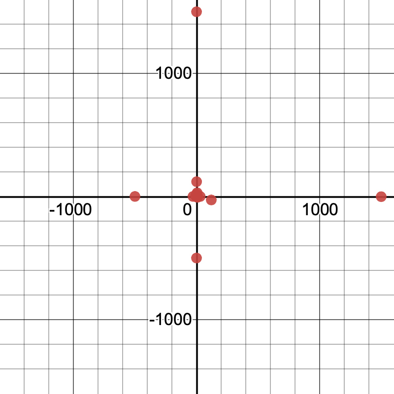
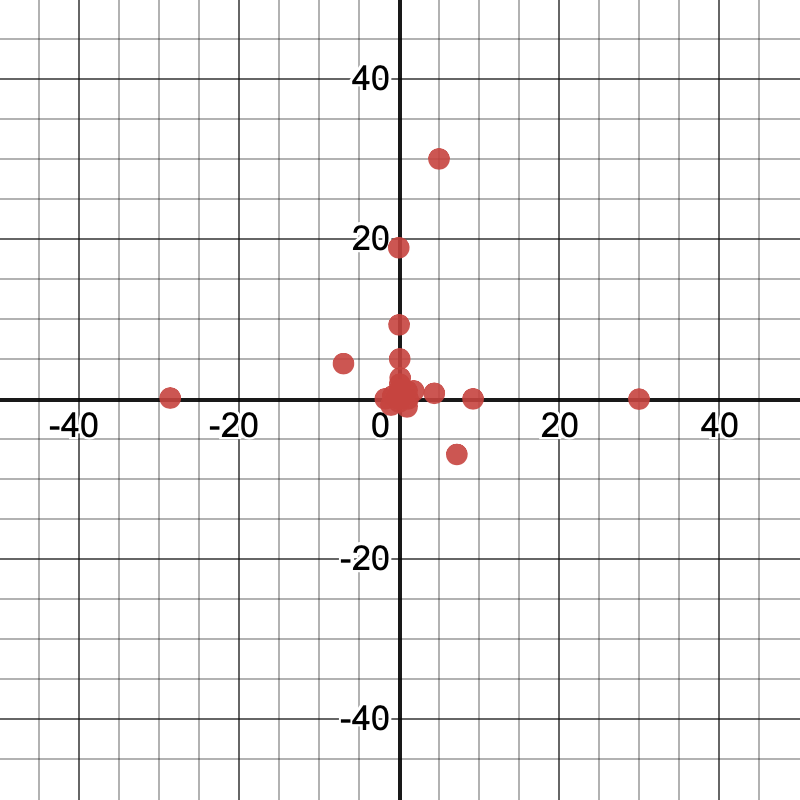
Here’s a corresponding table listing each of the guesses:
| a | b |
|---|---|
| 0 | 0 |
| 1 | 1 |
| -6.94 | 4.414 |
| 0.7 | 120 |
| -28.6 | 0.105 |
| 1.84 | 1 |
| -1 | -0.777 |
| 0.373 | 0.2 |
| 1500 | -1.71 |
| 0.0113 | 9.26 |
| 0.007 | -0.0081 |
| -500 | 0.06 |
| 1.13 | 0.0004 |
| -0.4 | 0.089 |
| 5 | 30 |
| -0.03 | 18.9 |
| 0.149 | 2.61 |
| 7.23 | -6.94 |
| 4.414 | 0.7 |
| 120 | -28.6 |
| 0.105 | 1.84 |
| 1 | -1 |
| -0.777 | 0.373 |
| 0.2 | 1500 |
| -1.71 | 0.0113 |
| 9.26 | 0.007 |
| -0.0081 | -500 |
| 0.06 | 1.13 |
| 0.0004 | -0.4 |
| 0.089 | 5 |
| 30 | -0.03 |
A few things to notice:
- There are some fairly small values and some fairly large values. The values span several orders of magnitude, from
$0.0004$to$1500$. - There are about as many values between
$0$and$1$as between$1$and$1500$. - There are some positive values and some negative values, with a small bias toward positive values.
- The values of the two parameters are not strongly correlated. In fact, the same sets of different values are used for each parameter, but their orders are chosen differently to avoid strong correlations.
- The calculator always tries all
$1$s and all$0$s. - There aren’t many other patterns besides these. The values aren’t actually random—the calculator always uses the same initial guesses for a given problem to try to avoid giving two different answers to two different people—but they aren’t highly structured either.
These properties reflect a compromise. The calculator generally doesn’t start with any knowledge about what’s reasonable in a specific problem, so its guesses are designed to work generically across a range of typical problems. Often, this works out pretty well, but not always. In particular, the calculator may struggle with problems that require some of the parameters to be extremely small or extremely large, or with problems where some of the parameters must take on very particular values before small changes in the parameters start pointing the way to the best global solution.
Recommended Workarounds
In the years since the calculator first gained the ability to do regressions, we started to notice some patterns in the problems that teachers and students reported that the calculator handled poorly, and we developed some advice to help in many of these situations:
Add a restriction on one of the parameters
If the calculator arrives at a solution that doesn’t make sense, you can use a domain restriction on one or more parameters to force the calculator to pick a different solution. For example, in the trig problem from the introduction, adding the restriction $\{0 \le b \le \pi\}$ was enough to guide the calculator to pick the desired low-frequency solution:
 restricted.png)
Change the units of the data
In many problems, there’s some freedom to choose what units the data are measured in. Using different units will often change the numerical values of the best fit parameters without changing the meaning of the fitted model. In these problems, it may help to choose units that make the best fit parameters not too large or too small.
Returning to the logistic fit from the introduction, measuring time in “years since 1900” instead of “years” reduces the best fit value of $b$ from $3.2 \cdot 10^{23}$ to $2.4$, which allowed the calculator to successfully find it.
 workaround.png)
The effect of changing units is especially pronounced in problems involving exponential functions because exponentials have a way of turning shifts in the inputs that are merely large into changes in the output that are unfathomably huge.
Restricting parameters and changing units are still useful bits of advice, and there’s now a help article on that for reference. But this advice hasn’t been so easy to discover the first time you need it, and it asks the user to do work that we’d really rather have the calculator do for us. Applying this advice automatically in some important cases has been the theme of most of the regressions improvements that we have made over the last year.
New Automated Strategies
The calculator has four new strategies that it can apply to special nonlinear regression problems to improve the chances of finding the best possible fit.
Account for simple parameter restrictions in initial guesses
Adding a parameter restriction like $\{0 \le b \le \pi\}$ has always worked for forcing the calculator to discard an undesirable solution, but it hasn’t always been as effective as you might hope in guiding the calculator to a good solution. The problem was that such restrictions had the effect of filtering initial guesses: any guess that didn’t satisfy the restrictions was immediately discarded leaving fewer total guesses to try. In fact, if a restriction was so tight that no initial guess satisfied it, the calculator couldn’t even get started and it would simply give up.
 over-restricted.png)
Now, the calculator is able to recognize simple restrictions and choose all its initial guesses to automatically satisfy them. Simple restrictions are restrictions that depend on only a single parameter and that are linear in that parameter. For example, $\{a > 0\}$ and $\{2 \lt b \lt 3\}$ are considered simple, but $\{ab > 0\}$ and $\{1/a \le 10\}$ are not. More complex restrictions are still allowed—they just continue to cause initial guesses to be filtered rather than remapped.
Automatically generate new parameter restrictions in special problems
Some regression problems have special symmetries that produce many solutions with exactly the same error. For example, in the trigonometric regression problem
y_1 \sim a \sin(bx_1 + c),
adding any multiple of $2\pi$ to $c$ (the phase) will have no effect on the errors. Similarly, simultaneously negating $a$, $b$, and $c$ leaves the errors unchanged.
If the data, $x_1$, is evenly spaced, there’s a much less obvious symmetry: if $D$ is the spacing between the data points, adding $2\pi/D$ to $b$ (the angular frequency) will have no effect on the errors. This means that there are an infinite set of models with different frequencies that all fit the data exactly equally as well.
We want the lowest frequency that will work, so the calculator now automatically synthesizes the restriction $\{0 \lt b \lt \pi/D\}$ in this problem internally (if you noticed a missing factor of two, it’s because this restriction also accounts for the negation symmetry mentioned previously). This synthesized restriction is linear in $b$, and so it influences the initial guesses for $b$ the same way a manually entered restriction would.
Aside: The phenomenon that discretely sampling a high-frequency signal can produce exactly the same results as sampling a lower frequency signal is known as aliasing. It has many important consequences for digital signal processing.
When the data represented by $x_1$ are not evenly spaced, the story is more complicated. The errors are still periodic in the angular frequency $b$, but the period is a complicated function of the data, and it can grow very large. In this case, the calculator does something that’s not quite rigorous: it adds an internal restriction based on the average spacing of the data. In practice, this seems to help much more often than it hurts, but there’s an escape hatch for cases where this heuristic is wrong: if there are any manually entered restrictions on a parameter, the calculator will not generate its own restrictions for that parameter. So a manual restriction can be used to choose a higher frequency solution than the calculator found.
Another common model with an important symmetry is the exponential model
y_1 \sim ab^{x_1}.
If all the data points represented by $x_1$ are even integers, then negating $b$ has no effect on the errors. But away from even integers, $b^x$ and $(-b)^x$ are very different functions, and the negative base solution is usually undesirable. To account for this, the calculator now automatically synthesizes the restriction $\{b \ge 0\}$ in this problem. This happens even when not all of the $x_1$ data points are even integers. Again, this seems to help much more often than it hurts, but again, if you do want a negative base solution, you can use the escape hatch of writing a manual restriction.
Solve for linear parameters exactly at every step
The calculator has always detected regression problems where all the parameters are linear and has used a special algorithm to solve for the parameters in a single step by solving a single linear algebra problem. But in many problems where some of the parameters are nonlinear, there are other parameters that are linear.
For example, in
y_1 \sim ab^{x_1} + c,
$a$ and $c$ are linear even though $b$ is not. The calculator now detects this special structure and uses it to solve exactly for the optimal values of linear parameters (holding the nonlinear parameters fixed) after every update to the nonlinear parameters.
There is one important but subtle point in implementing this idea. When considering derivatives of the error with respect to the parameters as part of a nonlinear update step, it’s important to take into account that the optimal values of the linear parameters are themselves functions of the nonlinear parameters. The algorithm that correctly takes this into account is called Variable Projection, and we benefitted from two papers describing this algorithm.
Solving exactly for linear parameters means that the calculator’s initial guesses for them are no longer important, and in many problems, it means that the units used to measure the $y$ data no longer matter. In problems of the form
y_1 \sim a f(x_1, u, v, ...),
rescaling the data represented by $y_1$ can be compensated by changing the value of the linear parameter $a$, and this is now accounted for at every step. Similarly, in problems of the form
y_1 \sim f(x_1, u, v, ...) + b,
a shift of the data represented by $y_1$ can be compensated by changing the value of the linear parameter $b$, and this is similarly accounted for at every step.
Automatically rewrite models in special problems
Sometimes there are several equivalent ways to write down a given model, but some ways are easier for the regression routine to work with than others. In some problems, the calculator now automatically rewrites the model internally, finds best fit parameters for the rewritten model, and then solves for the user-specified parameters in terms of the internal parameters.
For example, the calculator now rewrites
y_1 \sim a \sin(bx_1 + c)
as
y_1 \sim u \cos(bx_1) + v \sin(bx_1).
The latter form is easier to optimize because it has two linear parameters ($u$ and $v$) and one nonlinear parameter ($b$), whereas the original problem has only one linear parameter and two nonlinear parameters.
The calculator also rewrites several forms of exponential models internally. For example, the model
y_1 \sim \exp(mx_1 + b)
is rewritten to
y_1 \sim \exp\left(u \left(\frac{x_1 - c}{r}\right) + v\right),
where $c$ is a measure of the center of the $x_1$ data and $r$ is a measure of its scale (we use the midrange and range, but the mean and standard deviation would probably work just as well). This has the effect of making the fitting procedure work equally as well no matter what units the user chooses for $x_1$.
Notice how this strategy is complementary to the previous strategy: solving exactly for linear parameters at every step makes regressions more robust to different choices of units for the $y$ data, and this rewrite rule for exponential models makes regressions more robust to different choices of units for the $x$ data.
Similar rewrites apply to several other ways of writing exponential models, like
\begin{aligned}
y_1 & \sim ab^{x_1} \\
y_1 & \sim a \exp(bx_1) \\
y_1 & \sim a \cdot 2^{bx_1}
\end{aligned}
to make the fitting procedure for all of these forms independent of an overall shift or scale in the $x_1$ data.
In a logistic model, the denominator has an exponential part:
y_1 \sim \frac{a}{1 + b \exp(-c x_1)}
and these same rewrites are applied to that exponential subexpression and are helpful for the same reasons. Our testing suggests that logistic models benefit even more from this strategy than exponential models do, likely because logistic models are somewhat harder to fit in the first place.
These rewrites have one additional benefit: they can help us notice cases where the true best-fit parameters are too large or too small for the calculator to accurately represent. In this case, the calculator now gives the user a warning that links to a new help article.
Conclusion
If you have been using regressions in the Desmos Graphing Calculator, I hope your experiences have been largely positive. I think the system for defining and solving regression problems in Desmos is among the most flexible that I have seen, and is by far the fastest to use. But, in some cases, the calculator has not been able to find the best possible solution to nonlinear regression problems, even when it seems visually obvious that there must be a better solution. If you have run into problems like this and have been frustrated, I hope you’ll give regressions in the calculator another look. In my experience, the four new regression strategies implemented over the last year—using parameter restrictions to improve initial guesses, automatically generating parameter restrictions in special problems, solving for linear parameters at every step, and reparameterizing certain problems to make them easier to solve—combine to produce a major improvement in the robustness of the regression system.